Data for Equity
One convenient aspect of our data from the standpoint of beneficence is that we gather data at the city-level, so identification of persons is not an issue, and therefore we do not jeopardize anyone’s privacy. Our main goal with these datasets is to deduce what aspects of a city make it a better place to live than others. We recognize the need to consider how publication could reinforce social inequities, and we will take into account those issues which specifically affect the most vulnerable, so as not to leave them behind for the sake of “livability.” For example, it is crucial to take into account factors such as the proportion of a city’s population which lives in slums or does not have access to water in order to ensure that we do not draw conclusions which would encourage the further marginalization of those who are least fortunate in the societies we examine. Moreover, it is our hope that we can draw conclusions which would help cities better foster the inclusion of marginalized people; in other words, we hope to identify trends in the data which would indicate ways in which cities could reduce social inequality. To do so, researchers using our data could foster dialogue with marginalized communities identified in order to see if they share our conclusions; and if not, why they do not.
From the standpoint of justice, our data was collected from national governments, United Nations agencies, civil society organizations, and academic institutions, so we can be reasonably confident that no undue burden was put upon the people of the various countries in order to collect data. Again, the data is anonymous and high level- we do not use any data of individual persons, only population statistics/percentages, so we can be sure that our publication will not cause harm to any individuals/groups, and only help others in identifying and reducing inequality.
Considering that our conclusion will be based on the data sets that we have chosen, some limitations to the analysis we will do would be a certain degree of inaccuracy that may occur as a result of the missing values that were removed in the process of cleaning our data sets or even the fact that most of our data is taken from the past, with the most recent being 2019. Since beyond that year there have been major changes that have occurred in the world, primarily COVID-19, the conclusions of our analyses may not be as accurate as we would like it to be. Some abuse or misuse of the data that we use include the overlooking of this fact, that despite the limitations we’ve identified, we still insist on an inference or insight that is seemingly flawless, which may in turn lead to false or inaccurate information.
Loading Data Sets
#load datasets
load("air_q_by_c.RData")
load("slum_population.RData")
load("population.RData")
#load("water_q_avg.RData")
#load("combined.RData")
Urban Populations and Population Living in Slums
cols.num <- c("1990", "1995", "2000", "2005", "2010", "2014")
slum_pop_2[cols.num] <- sapply(slum_pop_2[cols.num],as.numeric)
slum_and_total_pop <- inner_join(x = slum_pop_2, y = urban_pop, by = c("Country" = "Region, subregion, country or area")) %>%
  select("Country", `2000.x`, `2005.x`, `2010.x`, `2000.y`, `2005.y`, `2010.y`) %>%
  pivot_longer(cols = `2000.x` : `2010.y`, names_to = "Year", values_to = "Population") %>%
  separate(col = Year, into = c("Year", "Group"), sep = "\\.") %>%
  mutate(Group = case_when(Group == "x" ~ "Slum",
                           Group == "y" ~ "Urban"))
slum_and_total_pop %>%
  ggplot() + facet_grid(~Year) +
    geom_bar(aes(y = Country, x = Population, fill = Group), position = 'dodge', stat= 'identity')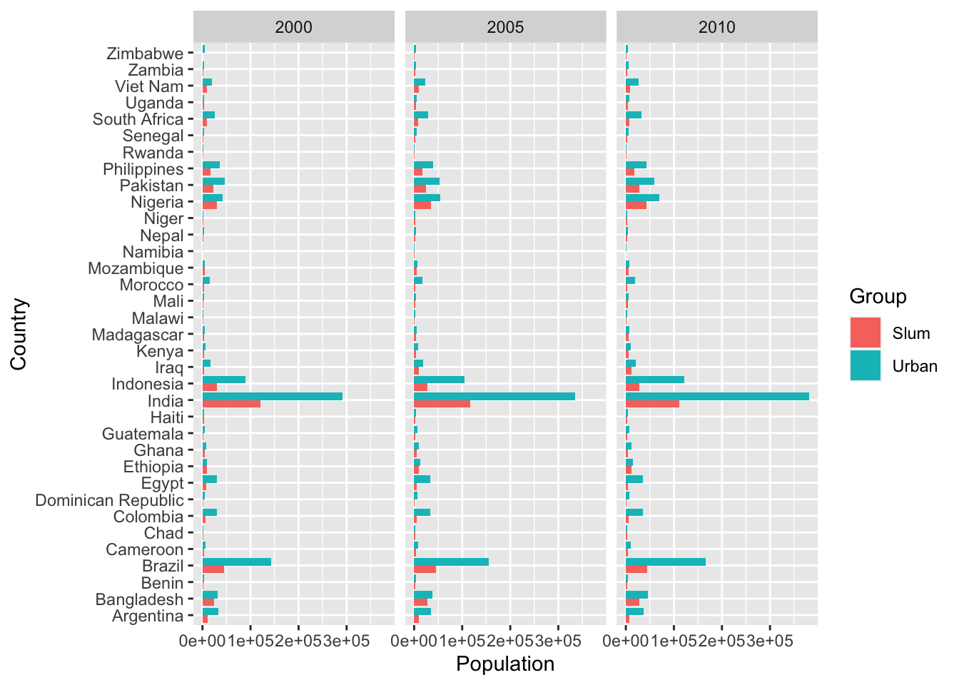
slum_and_total_pop %>%
pivot_wider(names_from = Group, values_from = Population) %>%
mutate(Prop_slum = Slum / Urban) %>%
ggplot() +
geom_line(aes(x = as.numeric(Year), y = Prop_slum, color = Country)) +
scale_x_continuous(breaks = c(2000, 2005, 2010)) +
labs(x = "Year", y = "Proportion of Urban Population in Slums", title = "Proportion of Urban Population Living in Slums", subtitle = "2000, 2005, 2010")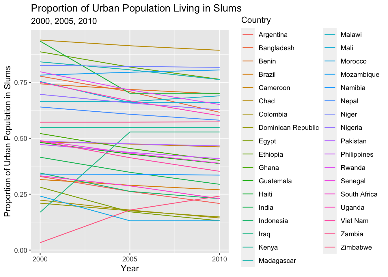 These graphs compare the urban population to the population living in slums for 35 countries. The first figure demonstrates that the slum population is much smaller than the urban population, but is hard to interpret because the India bar is so tall that all the other bars are barely visible. The second graph compares the proportion of the urban population living in slums for the same 35 countries for the years 2000, 2005, 2010, and although countries can’t be easily identified in this figure it is clear that for most the % slum population has been steady. Future directions with this data include identifying countries where the slum population is increasing or decreasing and try to identify possible reasons for this change.
Combining Cleaned Data Sets
colnames(urban_pop)[1] <- "Country"
pop <- urban_pop[-2]

water_quality <- read_csv("water_quality.csv")
water_quality <- water_quality %>% select(3,4,5,17,18,26,27,29:35) %>% rename(Country = 1, Region = 2, Year = 3, improved_water = 4, drinking_access = 5, improved_san = 6, san_access = 7, durable_1 = 8, durable_2 = 9, durable_3 = 10,  living_area = 11, phone_access = 12, cell_access = 13, electric_access = 14)
water_quality <- water_quality[-c(1, 2, 3, 4), ]
water_quality[,4:14] <- lapply(water_quality[,4:14], as.double)
water_quality_cols <- colnames(water_quality)[4:14]
water_quality_avg <- water_quality %>%
  group_by(Country) %>%
  top_n(1,Year)

water_quality_avg_clean <- na.omit(aggregate(cbind(improved_water, drinking_access, improved_san, san_access, durable_1, durable_2, durable_3, living_area, phone_access, cell_access, electric_access)~Country, water_quality_avg, mean, na.rm=TRUE, na.action=na.pass))

water_quality_avg_clean
## Country improved_water drinking_access improved_san
## 1 Afghanistan 96.45000 62.55000 71.35000
## 2 Albania 99.40000 97.50000 99.10000
## 3 Angola 95.90000 71.20000 97.30000
## 6 Azerbaijan 99.50000 81.60000 98.40000
## 9 Belize 95.55000 96.80000 97.90000
## 11 Bolivia 93.53333 27.36667 77.78889
## 12 Bosnia and Herzegovina 99.60000 99.60000 98.95000
## 18 Cameroon 92.80000 86.60000 88.40000
## 19 Central African Republic 96.40000 56.00000 95.70000
## 20 Chad 99.80000 91.20000 69.80000
## 22 Comoros 99.90000 85.90000 26.60000
## 23 Congo 98.10000 92.90000 79.65000
## 24 Congo DRC 99.20000 84.30000 64.10000
## 25 Costa Rica 99.73333 99.75000 97.35000
## 26 Cote d'Ivoire 99.70000 1.90000 90.00000
## 30 Ethiopia 99.70000 75.80000 81.60000
## 31 Gabon 98.40000 69.50000 77.10000
## 33 Georgia 100.00000 100.00000 99.90000
## 34 Ghana 99.65000 97.43333 94.30000
## 35 Guatemala 99.40000 82.27500 92.02500
## 37 Guinea Bissau 91.66667 78.46667 32.93333
## 39 Haiti 99.10000 92.40000 85.10000
## 41 India 98.47143 87.70000 86.40000
## 43 Iraq 51.75000 51.75000 97.10000
## 45 Kazakhstan 84.70000 99.40000 99.90000
## 46 Kenya 98.40000 97.80000 92.70000
## 48 Lao People's Democratic Republic 93.46667 93.30000 89.86667
## 49 Lesotho 99.00000 90.90000 95.30000
## 52 Malawi 99.40000 95.00000 57.90000
## 53 Maldives 99.30000 34.10000 99.90000
## 54 Mali 98.90000 93.10000 93.60000
## 59 Mozambique 100.00000 99.40000 94.50000
## 60 Myanmar 97.05000 87.70000 86.15000
## 61 Namibia 97.70000 85.10000 89.10000
## 63 Nicaragua 98.30000 70.00000 81.00000
## 64 Niger 97.30000 86.00000 84.40000
## 65 Nigeria 93.43333 90.05000 73.56667
## 67 Pakistan 84.53333 79.30000 93.73333
## 69 Papua New Guinea 98.80000 97.80000 86.20000
## 70 Paraguay 99.55000 72.05000 95.20000
## 71 Peru 95.01111 93.70000 87.27778
## 73 Rwanda 96.90000 88.30000 94.10000
## 76 Serbia 99.90000 99.20000 99.00000
## 77 Sierra Leone 93.70000 81.30000 86.30000
## 82 Tanzania 96.70000 95.85000 93.80000
## 84 Timor-Leste 99.00000 97.60000 89.50000
## 86 Trinidad and Tobago 96.51667 43.80000 97.28333
## 88 Turkmenistan 100.00000 100.00000 100.00000
## 89 Uganda 98.70000 97.30000 86.60000
## 95 Yemen 99.16667 52.00000 93.76667
## 96 Zambia 98.60000 90.60000 87.70000
## 97 Zimbabwe 98.55000 96.25000 98.20000
## san_access durable_1 durable_2 durable_3 living_area phone_access
## 1 58.75000 90.45000 58.40000 32.80000 54.65000 4.700000
## 2 98.10000 99.90000 99.70000 99.30000 93.70000 30.500000
## 3 71.80000 94.50000 96.20000 99.20000 67.50000 5.500000
## 6 85.10000 29.00000 97.50000 99.80000 79.60000 86.200000
## 9 94.60000 73.95000 83.10000 99.40000 87.70000 16.800000
## 11 55.10000 71.35556 87.53333 96.27778 68.23333 29.777778
## 12 98.90000 82.50000 98.20000 96.80000 97.90000 92.500000
## 18 63.80000 85.90000 86.40000 96.30000 77.96667 2.233333
## 19 48.50000 45.40000 70.10000 97.60000 98.30000 2.800000
## 20 32.20000 37.80000 73.40000 98.80000 58.50000 3.800000
## 22 22.40000 74.80000 86.10000 98.30000 82.70000 15.200000
## 23 31.00000 93.90000 90.45000 98.95000 83.20000 3.500000
## 24 20.70000 93.20000 92.60000 99.70000 51.00000 2.700000
## 25 94.81667 94.58333 92.40000 98.26667 94.63333 63.083333
## 26 60.40000 99.20000 95.20000 95.30000 100.00000 5.800000
## 30 29.00000 94.00000 35.40000 97.70000 66.90000 30.500000
## 31 47.00000 96.80000 100.00000 99.70000 75.60000 3.100000
## 33 96.50000 99.30000 97.80000 99.50000 87.00000 78.500000
## 34 24.00000 98.86667 96.80000 99.63333 69.23333 2.500000
## 35 79.60000 90.90000 89.67500 99.60000 73.25000 18.875000
## 37 19.40000 68.96667 17.26667 94.70000 76.30000 1.166667
## 39 49.20000 94.80000 93.50000 96.30000 63.30000 1.100000
## 41 69.57143 84.68571 90.61429 95.44286 68.67143 7.400000
## 43 75.00000 97.53333 87.73333 94.46667 56.76667 37.633333
## 45 98.00000 99.20000 94.30000 99.90000 96.10000 91.800000
## 46 55.80000 99.70000 67.70000 100.00000 77.20000 2.700000
## 48 84.76667 93.83333 87.63333 97.16667 78.23333 32.233333
## 49 45.10000 95.30000 95.60000 97.50000 78.90000 9.400000
## 52 31.40000 83.00000 86.50000 91.60000 82.80000 4.700000
## 53 97.50000 98.80000 98.40000 99.60000 61.30000 48.200000
## 54 58.20000 83.65000 94.35000 98.45000 84.10000 7.850000
## 59 85.00000 96.60000 98.00000 99.50000 86.30000 4.500000
## 60 68.30000 62.20000 55.75000 98.60000 69.65000 12.050000
## 61 67.70000 91.10000 86.70000 87.10000 81.40000 39.400000
## 63 75.10000 77.60000 81.80000 99.30000 59.50000 28.200000
## 64 33.90000 83.30000 56.90000 67.00000 61.10000 7.000000
## 65 38.93333 74.53333 91.48333 97.72500 68.66667 1.050000
## 67 86.96667 88.20000 86.70000 83.20000 44.23333 12.566667
## 69 71.00000 98.60000 89.30000 99.10000 52.70000 13.200000
## 70 90.15000 94.80000 96.85000 98.85000 89.70000 34.250000
## 71 76.67778 70.32222 61.72222 90.17778 82.06667 34.077778
## 73 40.60000 83.70000 82.20000 98.80000 89.60000 0.800000
## 76 97.20000 99.90000 99.10000 98.90000 97.70000 92.600000
## 77 32.60000 83.90000 95.50000 87.50000 53.20000 0.200000
## 82 50.20000 87.75000 85.50000 99.00000 85.60000 2.250000
## 84 77.20000 90.40000 69.60000 97.20000 77.30000 12.600000
## 86 93.71429 78.50000 91.04286 99.82500 95.11429 69.557143
## 88 99.20000 100.00000 100.00000 100.00000 93.80000 97.300000
## 89 31.60000 98.30000 94.60000 99.00000 55.20000 6.400000
## 95 91.96667 97.80000 98.50000 51.33333 52.86667 42.900000
## 96 31.90000 97.60000 98.80000 99.80000 66.80000 3.900000
## 97 57.55000 96.65000 97.85000 99.20000 81.00000 13.650000
## cell_access electric_access
## 1 96.20000 91.35000
## 2 99.10000 0.00000
## 3 94.90000 82.30000
## 6 77.50000 99.50000
## 9 96.70000 98.00000
## 11 77.96667 96.58889
## 12 70.50000 100.00000
## 18 95.56667 87.56667
## 19 91.70000 46.90000
## 20 94.90000 54.80000
## 22 93.70000 85.10000
## 23 97.20000 85.70000
## 24 95.90000 90.40000
## 25 94.03333 99.66000
## 26 97.40000 97.30000
## 30 97.50000 99.80000
## 31 98.30000 99.50000
## 33 76.00000 98.60000
## 34 97.70000 94.20000
## 35 93.22500 97.67500
## 37 97.46667 29.23333
## 39 92.90000 88.80000
## 41 97.37143 98.60000
## 43 78.13333 99.80000
## 45 99.00000 99.95000
## 46 99.60000 97.90000
## 48 96.56667 95.80000
## 49 95.90000 67.90000
## 52 86.90000 65.40000
## 53 99.60000 99.90000
## 54 98.40000 91.00000
## 59 97.80000 97.30000
## 60 96.05000 97.05000
## 61 87.70000 86.80000
## 63 21.50000 99.50000
## 64 89.30000 73.50000
## 65 95.76667 79.90000
## 67 97.36667 98.76667
## 69 94.60000 87.70000
## 70 98.65000 99.85000
## 71 90.84444 97.25556
## 73 93.90000 91.50000
## 76 97.70000 100.00000
## 77 96.80000 62.80000
## 82 97.00000 70.00000
## 84 98.30000 98.90000
## 86 88.00000 97.61429
## 88 100.00000 100.00000
## 89 98.70000 95.10000
## 95 95.96667 99.40000
## 96 92.70000 78.60000
## 97 97.30000 88.15000slum_pop_2[,2:9] <- lapply(slum_pop_2[,2:9], as.double)
combined_data <- air_quality_by_country %>%
##inner_join(slum_pop_2, by="Country") %>%
inner_join(pop, by="Country") %>%
inner_join(water_quality_avg_clean, by="Country")
head(combined_data)## Country 2015.x 2016 2017 2018 2019 2000 2005
## 1 Afghanistan 59.98571 56.56000 52.74857 52.13143 51.69429 4436 5692
## 2 Albania 19.37500 17.62500 18.80000 18.60000 18.40000 1303 1439
## 3 Azerbaijan 25.51667 23.88333 24.47500 24.41667 24.61667 4174 4473
## 4 Belize 21.25714 20.42857 20.15714 20.42857 20.34286 112 128
## 5 Bosnia and Herzegovina 33.80000 29.56667 30.80000 30.80000 30.33333 1596 1663
## 6 Cameroon 69.33636 65.17273 62.25455 63.88182 64.54545 6956 8456
## 2010 2015.y 2020 2025 2030 2035 2040 2045 2050 improved_water
## 1 6837 8368 9904 11705 13818 16279 19104 22228 25499 96.45
## 2 1534 1679 1827 1949 2038 2090 2106 2102 2083 99.40
## 3 4824 5262 5696 6101 6491 6883 7253 7572 7833 99.50
## 4 145 163 183 205 230 256 283 311 338 95.55
## 5 1696 1668 1715 1768 1824 1876 1919 1952 1976 99.60
## 6 10297 12463 14942 17740 20857 24291 28049 32106 36415 92.80
## drinking_access improved_san san_access durable_1 durable_2 durable_3
## 1 62.55 71.35 58.75 90.45 58.4 32.8
## 2 97.50 99.10 98.10 99.90 99.7 99.3
## 3 81.60 98.40 85.10 29.00 97.5 99.8
## 4 96.80 97.90 94.60 73.95 83.1 99.4
## 5 99.60 98.95 98.90 82.50 98.2 96.8
## 6 86.60 88.40 63.80 85.90 86.4 96.3
## living_area phone_access cell_access electric_access
## 1 54.65000 4.700000 96.20000 91.35000
## 2 93.70000 30.500000 99.10000 0.00000
## 3 79.60000 86.200000 77.50000 99.50000
## 4 87.70000 16.800000 96.70000 98.00000
## 5 97.90000 92.500000 70.50000 100.00000
## 6 77.96667 2.233333 95.56667 87.56667Relationship Between Access to Sanitation and Electricity
combined_data %>%
ggplot(aes(x=electric_access, y=san_access)) + geom_point(aes(color = Country)) +
theme(legend.text = element_text(size=5), legend.spacing.y = unit(.001, 'cm'), legend.spacing.x = unit(.1, 'cm')) + labs(y="Access to Sanitation", x="Access to Electricity") +
geom_smooth(method="lm")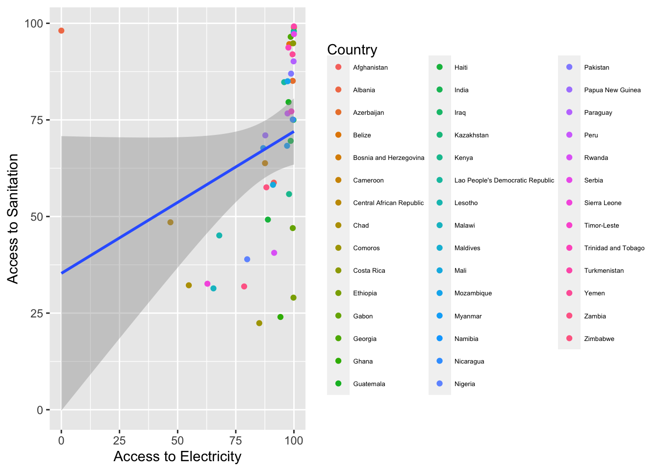 Here, we try to investigate the possible relationships between access to electricty and access to sanitation in different countries. It may seem at first glance that the two are somewhat unrelated, but from the plot, we can see that there exists some relationship between the two variables – countries with better access to electricity tend to have better access to sanitation as well. However, it is important to note that the relationship between the two variables in question do not necessarily have a causal relationship. With that being said, there is a slight positive linear correlation between access to sanitation and access to electricity.
Relationship Between Drinking Access and Improved Water Quality
combined_data %>%
ggplot(aes(x=drinking_access, y=improved_water)) + geom_point(aes(color=Country)) +
theme(legend.text = element_text(size=5), legend.spacing.y = unit(.001, 'cm'), legend.spacing.x = unit(.1, 'cm')) + geom_smooth(method="lm")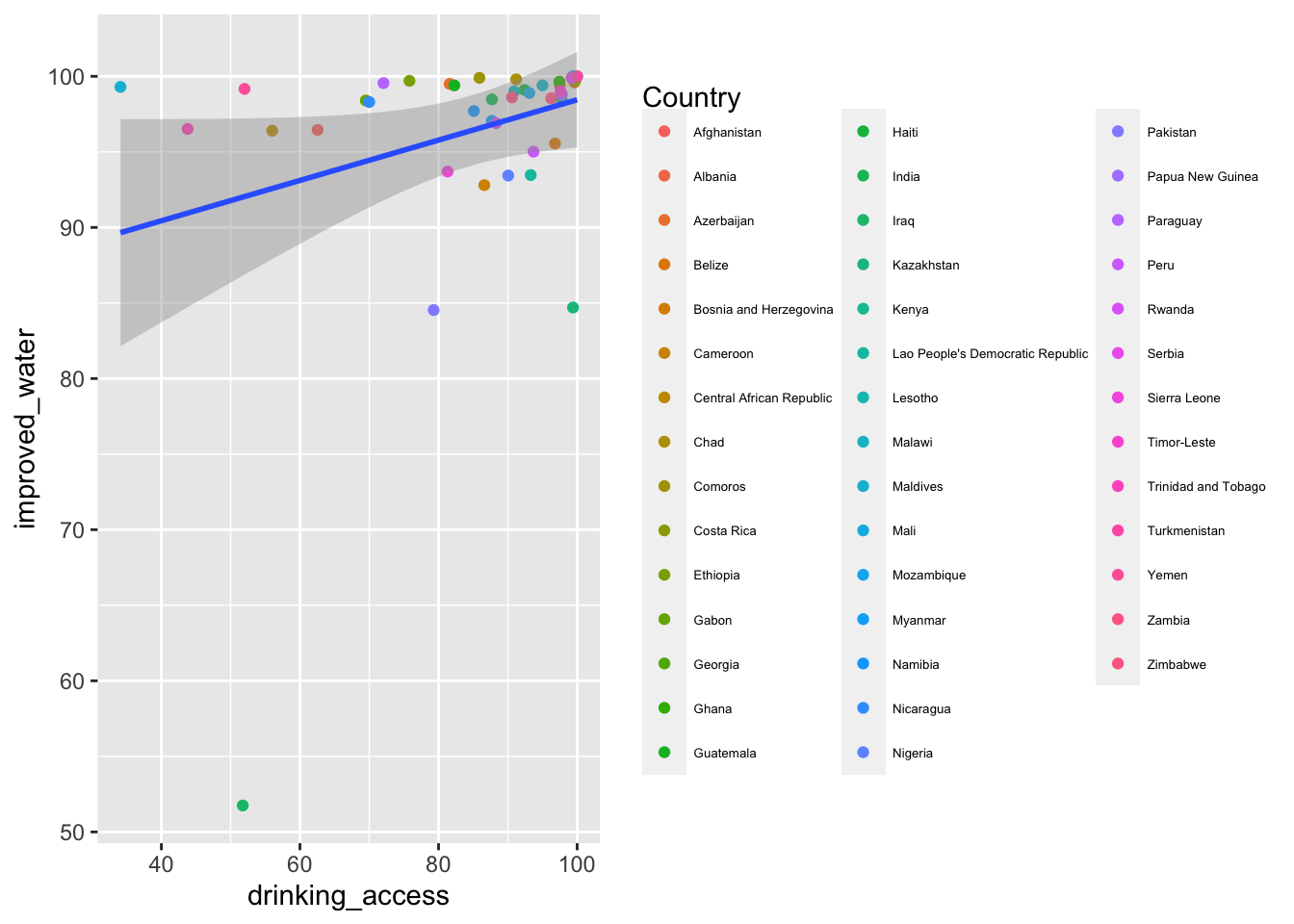 Looking at the relationship between drinking access of a country and improved water quality, we can see that the figure shows a potential correlation between the two variables. On the other hand, we can also see that the fitted line does not describe the data set very accurately as there are evidently outliers. With this said, there exists a slight positive relationship between drinking access and improved water quality, which is intuitively expected. Similarly to the previous graph, it is inaccurate to assume that the two variables have a causal relationship but may be more plausible to say that the two are correlated to a certain degree.