Data Loading and Cleaning
Air Quality Dataset
air_quality <- read_csv("air_quality.csv", skip = 2)
air_quality$`Subnational Regions` <- NULL
air_quality$`Data Units` <- NULL
air_quality$"2015" = as.numeric(as.character(air_quality$"2015"))
air_quality$"2016" = as.numeric(as.character(air_quality$"2016"))
air_quality$"2017" = as.numeric(as.character(air_quality$"2017"))
air_quality$"2018" = as.numeric(as.character(air_quality$"2018"))
air_quality$"2019" = as.numeric(as.character(air_quality$"2019"))
air_quality_by_country <- aggregate(air_quality[,2:6], air_quality[,1], FUN = mean)


air_quality_by_country_clean <- reshape(data = air_quality_by_country, direction = "long", idvar = "Country", varying = list(2:6), v.names = "Air_Quality", times = 2015:2019)

head(air_quality_by_country)
## Country 2015 2016 2017 2018 2019
## 1 Afghanistan 59.98571 56.56000 52.74857 52.13143 51.69429
## 2 Albania 19.37500 17.62500 18.80000 18.60000 18.40000
## 3 Algeria 34.83673 34.65918 34.20816 34.35714 34.53265
## 4 American Samoa 6.10000 6.60000 6.40000 6.40000 6.40000
## 5 Andorra 10.62500 9.21250 9.40000 9.47500 9.35000
## 6 Argentina 17.18400 16.44400 15.88800 15.88400 15.71200graph1 <- ggplot(air_quality_by_country_clean, aes(x = time, y = Air_Quality, color = Country)) + geom_line(show.legend = FALSE) + scale_x_continuous(breaks = 2015:2019)
graph1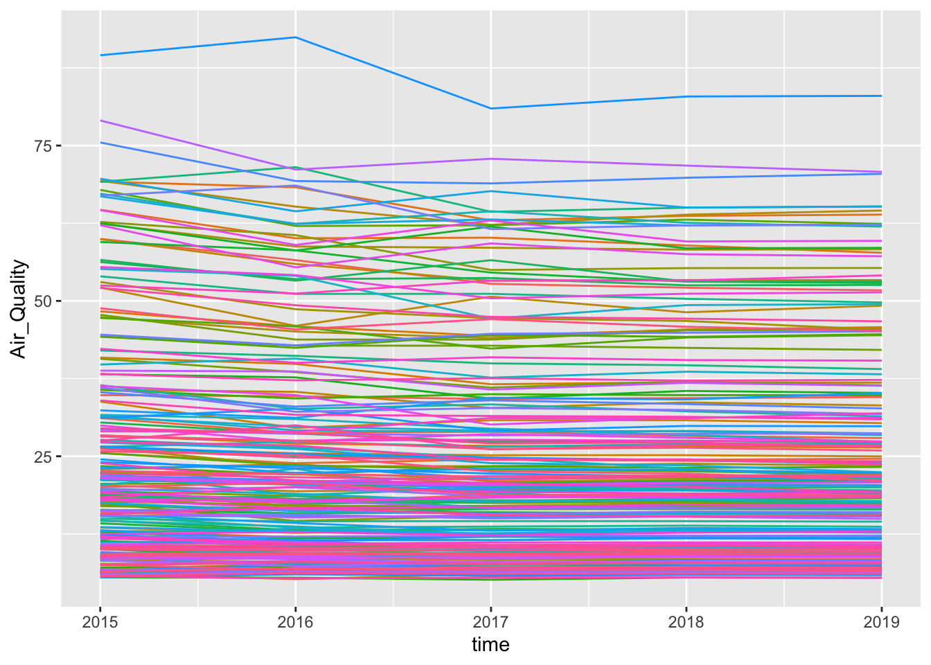
The air_quality csv file was somewhat clean to begin with, having only 2 columns to skip at the start and having 2 more columns regarding the region and the measurement used as the only different columns to remove. After removing the columns, I changed the years to be a double in order to group them by the country, and I used R’s aggregate function to get the mean air quality of a country. Afterwards, I reshaped the data in a way that it could be plotted and showed the graph. Since there are a lot of countries, the graph may be quite hard to see, so we plan to separate them by either their economic status or region to better visualize how impactful air quality is.
Slum Population Dataset
slum_population <- read_csv("slum_population.csv")
slum_population$Region <- NULL
slum_population$`Data Units` <- NULL
slum_pop_1 <- na.omit(slum_population)
head(slum_pop_1)
## # A tibble: 6 × 9
## `Country or area` `1990` `1995` `2000` `2005` `2010` `2014` `2016` `2018`
## <chr> <chr> <chr> <chr> <chr> <chr> <chr> <dbl> <dbl>
## 1 Benin 1,361 1,667 1,956 2,324 2,767 2,857 2993 3216
## 2 Cameroon 2,362 2,843 3,364 4,008 4,751 4,533 3499 3422
## 3 CAR 947 1,119 1,299 1,479 1,660 1,683 1819 1930
## 4 Chad 1,227 1,449 1,695 2,005 2,334 2,678 2851 3065
## 5 Cote d'Ivoire 2,575 3,254 3,979 4,662 5,501 6,188 6995 7733
## 6 Ethiopia 5,794 7,565 8,693 9,855 11,597 13,670 13413 14775slum_pop_2 <- filter(slum_pop_1, slum_pop_1$'Country or area'!="Palestine" & slum_pop_1$'Country or area'!='Cuba' & slum_pop_1$'Country or area'!='Maldives')
head(slum_pop_2)## # A tibble: 6 × 9
## `Country or area` `1990` `1995` `2000` `2005` `2010` `2014` `2016` `2018`
## <chr> <chr> <chr> <chr> <chr> <chr> <chr> <dbl> <dbl>
## 1 Benin 1,361 1,667 1,956 2,324 2,767 2,857 2993 3216
## 2 Cameroon 2,362 2,843 3,364 4,008 4,751 4,533 3499 3422
## 3 CAR 947 1,119 1,299 1,479 1,660 1,683 1819 1930
## 4 Chad 1,227 1,449 1,695 2,005 2,334 2,678 2851 3065
## 5 Cote d'Ivoire 2,575 3,254 3,979 4,662 5,501 6,188 6995 7733
## 6 Ethiopia 5,794 7,565 8,693 9,855 11,597 13,670 13413 14775sort(slum_pop_2$`Country or area`)## [1] "Argentina" "Bangladesh" "Benin"
## [4] "Bolivia" "Brazil" "Cameroon"
## [7] "CAR" "Chad" "Colombia"
## [10] "Cote d'Ivoire" "Dominican Republic" "Egypt"
## [13] "Ethiopia" "Ghana" "Guatemala"
## [16] "Haiti" "India" "Indonesia"
## [19] "Iraq" "Kenya" "Madagascar"
## [22] "Malawi" "Mali" "Morocco"
## [25] "Mozambique" "Namibia" "Nepal"
## [28] "Niger" "Nigeria" "Pakistan"
## [31] "Philippines" "Rwanda" "Senegal"
## [34] "South Africa" "Tanzania" "Uganda"
## [37] "Viet Nam" "Zambia" "Zimbabwe"Loading the slum population csv onto RStudio, there were some unnecessary columns such as Region and Data Units that we removed since it would be distracting to the future operations that would be done on this data set along with others. Since there were several null (NA) values found in the table, we also made sure that these values were taken out of the final data set that we would use. Furthermore, there were three countries – Palestine, Cuba, and the Maldives – that had values listed as “-” for all of the years in the data set. Consequently, we removed the data through the filter function as these values were not identified as null. At the end, we sorted the data set alphabetically by country name.
Population for Urban Areas Dataset
pop <- read_csv("population.csv", skip = 2) %>%
  mutate(across(.cols = starts_with("2"), ~ as.numeric(str_replace_all(.x, " ", "")))) %>%
  filter(!is.na(`2050`))
head(pop)
## # A tibble: 6 × 13
## `Region, subreg… Unit `2000` `2005` `2010` `2015` `2020` `2025` `2030` `2035`
## <chr> <chr> <dbl> <dbl> <dbl> <dbl> <dbl> <dbl> <dbl> <dbl>
## 1 WORLD Thou… 2.87e6 3.22e6 3.59e6 3.98e6 4.38e6 4.77e6 5.17e6 5.56e6
## 2 More developed … Thou… 8.84e5 9.18e5 9.54e5 9.79e5 1.00e6 1.03e6 1.05e6 1.07e6
## 3 Less developed … Thou… 1.98e6 2.30e6 2.64e6 3.00e6 3.38e6 3.75e6 4.12e6 4.49e6
## 4 Least developed… Thou… 1.66e5 2.05e5 2.50e5 3.06e5 3.72e5 4.49e5 5.39e5 6.39e5
## 5 Less developed … Thou… 1.82e6 2.09e6 2.39e6 2.70e6 3.00e6 3.30e6 3.58e6 3.85e6
## 6 Less developed … Thou… 1.50e6 1.71e6 1.95e6 2.20e6 2.47e6 2.76e6 3.07e6 3.40e6
## # … with 3 more variables: 2040 <dbl>, 2045 <dbl>, 2050 <dbl>Similarly, the population file was also cleaned by firstly skipping the 2 columns to get the right column headings. The population values were character vectors with spaces separating the numbers, so the whitespace in the strings had to be removed and then the characters converted to numeric values. This data set is particularly unique since there are estimates for populations for urban areas in the coming future for the years 2025 up to the year 2050.
Water Quality Dataset
water_quality <- read_csv("water_quality.csv")

water_quality <- water_quality %>% select(3,4,5,17,18,26,27,29:35) %>% rename(Country = 1, Region = 2, Year = 3, improved_water = 4, drinking_access = 5, improved_san = 6, san_access = 7, durable_1 = 8, durable_2 = 9, durable_3 = 10,  living_area = 11, phone_access = 12, cell_access = 13, electric_access = 14)

water_quality <- water_quality[-c(1, 2, 3, 4), ]
head(water_quality)
## # A tibble: 6 × 14
## Country Region Year improved_water drinking_access improved_san san_access
## <chr> <chr> <chr> <chr> <chr> <chr> <chr>
## 1 Angola Luanda 2006 100 16.4 93.8 <NA>
## 2 Angola Luanda 2011 99.1 <NA> 94.5 <NA>
## 3 Angola Luanda 2015 95.9 71.2 97.3 71.8
## 4 Benin Cotonou 1996 97.9 <NA> 71.7 <NA>
## 5 Benin Cotonou 2001 100 98.2 80.2 26
## 6 Benin Cotonou 2011 98.7 98.7 25.1 <NA>
## # … with 7 more variables: durable_1 <chr>, durable_2 <chr>, durable_3 <chr>,
## # living_area <chr>, phone_access <chr>, cell_access <chr>,
## # electric_access <chr>#water_quality <- aggregate(water_quality[,4:14], water_quality[,1:3], FUN = mean)The water_quality csv file includes information about the proportion of people in each country and region that have access to vital resources. The column names were spread over multiple rows, so I eliminated most of them and renamed them. I deleted some columns which had most/only NAs and kept the columns of important metrics, including improved water quality, sanitation, housing, and utility access data. However, the proportions represented data collected from a wide range of years, and the years were not consistent throughout each country or region.
Gini Dataset
read_csv("gini.csv", skip = 1) %>%
  mutate_all(~na_if(.x, y = ".."))
## # A tibble: 227 × 10
## Country `City/region` `2010` `2011` `2012` `2013` `2014` `2015` `2016` `2017`
## <chr> <chr> <chr> <chr> <chr> <chr> <chr> <chr> <chr> <chr>
## 1 Kazakh… Akmola 0.27 0.28 0.28 0.27 0.28 0.27 0.27 0.27
## 2 Kazakh… Aktobe 0.27 0.28 0.28 0.26 0.26 0.27 0.24 0.25
## 3 Kazakh… Almaty 0.26 0.25 0.25 0.25 0.25 0.26 0.26 0.28
## 4 Kazakh… Almaty City 0.24 0.26 0.25 0.25 0.25 0.27 0.29 0.29
## 5 Kazakh… Atyrau 0.22 0.23 0.21 0.21 0.21 0.22 0.23 0.23
## 6 Kazakh… City of Asta… 0.29 0.27 0.24 0.23 0.23 0.22 0.22 0.23
## 7 Kazakh… East Kazakhs… 0.28 0.29 0.28 0.28 0.28 0.28 0.28 0.31
## 8 Kazakh… Karaganda 0.27 0.29 0.31 0.29 0.29 0.29 0.29 0.30
## 9 Kazakh… Kostanai 0.26 0.26 0.26 0.27 0.27 0.25 0.26 0.25
## 10 Kazakh… Kyzylorda 0.23 0.26 0.24 0.23 0.22 0.21 0.20 0.24
## # … with 217 more rowsThe gini dataset reports the gini coefficient, a measure of income distribution across a population, by city and/or region between the years of 2010 - 2017. This dataset once again needed the first row skipped to have the correct column headings. This dataset has a lot of missing values, and “..” was used to denote missing values, so we replaced “..” with NA for easy filtering during data exploration.
Public Transport Dataset
read_csv("public_transport.csv", skip = 2)## # A tibble: 1,537 × 5
## Cities Country Region `Percentage Valu… `Estimate Source`
## <chr> <chr> <chr> <dbl> <chr>
## 1 Asyut Egypt Western Asia … 22.8 UN-Habitat Urban Indi…
## 2 Basel Switzerland Northern Ameri… 95.4 European Commission D…
## 3 Atbara Sudan Western Asia … 10.1 UN-Habitat Urban Indi…
## 4 Athina Greece Northern Ameri… 97.0 European Commission D…
## 5 Auckland New Zealand Australia and … 94.4 UN-Habitat Urban Indi…
## 6 Augsburg Germany Northern Ameri… 92.9 European Commission D…
## 7 Avignon France Northern Ameri… 92.1 European Commission D…
## 8 Avilés Spain Northern Ameri… 93.2 European Commission D…
## 9 Awassa Ethiopia Sub-Saharan Af… 38.5 UN-Habitat Urban Indi…
## 10 Ayacucho Peru Latin America … 26.3 UN-Habitat Urban Indi…
## # … with 1,527 more rowsLike many others, the Public Transport dataset needed the first two rows skipped for the correct column headings. This dataset lists the percentage of the population with easy access to public transportation for different cities.